Table of Contents
| DATA ANALYTICS REFERENCE DOCUMENT |
|
|---|---|
| Document Title: | Document Title |
| Document No.: | 1552735583 |
| Author(s): | Gerhard van der Linde, Rita Raher |
| Contributor(s): | |
REVISION HISTORY
| Revision | Details of Modification(s) | Reason for modification | Date | By |
|---|---|---|---|---|
| 0 | Draft release | Document description here | 2019/03/16 11:26 | Gerhard van der Linde, Rita Raher |
Week 8 - Sorting Algorithms Part 1
Overview
- Introduction to sorting
- Conditions for sorting
- Comparator functions and comparison-based sorts
- Sort keys and satellite data
- Desirable properties for sorting algorithms
- Stability
- Efficiency
- In-place sorting
- Overview of some well-known sorting algorithms
- Criteria for choosing a sorting algorithm
Sorting
- Sorting – arrange a collection of items according to some pre-defined ordering rules
- There are many interesting applications of sorting, and many different sorting algorithms, each with their own strengths and weaknesses.
- It has been claimed that as many as 25% of all CPU cycles are spent sorting, which provides a great incentive for further study and optimization
- The search for efficient sorting algorithms dominated the early days of computing.
- Numerous computations and tasks are simplified by properly sorting information in advance, e.g. searching for a particular item in a list, finding whether any duplicate items exist, finding the frequency of each distinct item, finding order statistics of a collection of data such as the maximum, minimum, median and quartiles.
Timeline of sorting algorithms
- 1945 – Merge Sort developed by John von Neumann
- 1954 – Radix Sort developed by Harold H. Seward
- 1954 – Counting Sort developed by Harold H. Seward
- 1959 – Shell Sort developed by Donald L. Shell
- 1962 – Quicksort developed by C. A. R. Hoare
- 1964 – Heapsort developed by J. W. J. Williams
- 1981 – Smoothsort published by Edsger Dijkstra
- 1997 – Introsort developed by David Musser
- 2002 – Timsort implemented by Tim Peters
Sorting
- Sorting is often an important step as part of other computer algorithms, e.g. in computer graphics (CG) objects are often layered on top of each other; a CG program may have to sort objects according to an “above” relation so that objects may be drawn from bottom to top
- Sorting is an important problem in its own right, not just as a preprocessing step for searching or some other task
- Real-world examples:
- Entries in a phone book, sorted by area, then name
- Transactions in a bank account statement, sorted by transaction number or date
- Results from a web search engine, sorted by relevance to a query string
Conditions for sorting
- A collection of items is deemed to be “sorted” if each item in the collection is less than or equal to its successor
- To sort a collection A, the elements of A must be reorganised such that if A[i] < A[j], then i < j
- If there are duplicate elements, these elements must be contiguous in the resulting ordered collection – i.e. if A[i] = A[j] in a sorted collection, then there can be no k such that i < k < j and A[i] ≠ A[k].
- The sorted collection A must be a permutation of the elements that originally formed A (i.e. the contents of the collection must be the same before and after sorting)
Comparing items in a collection
- What is the definition of “less than”? Depends on the items in the collection and the application in question
- When the items are numbers, the definition of “less than” is obvious (numerical ordering)
- If the items are characters or strings, we could use lexicographical ordering (i.e. apple < arrow < banana)
- Some other custom ordering scheme – e.g. Dutch National Flag Problem (Dijkstra), red < white < blue
Comparator functions
- Sorting collections of custom objects may require a custom ordering scheme
- In general: we could have some function compare(a,b) which returns:
- -1 if a < b
- 0 if a = b
- 1 if a > b
- Sorting algorithms are independent of the definition of “less than” which is to be used
- Therefore we need not concern ourselves with the specific details of the comparator function used when designing sorting algorithms
Inversions
- The running time of some sorting algorithms (e.g. Insertion Sort) is strongly related to the number of inversions in the input instance.
- The number of inversions in a collection is one measure of how far it is from being sorted.
- An inversion in a list A is an ordered pair of positions (i, j) such that:
- i < j but A[i] > A[j].
- i.e. the elements at positions i and j are out of order
- E.g. the list [3,2,5] has only one inversion corresponding to the pair (3,2), the list [5,2,3] has two inversions, namely, (5,2) and (5,3), the list [3,2,5,1] has four inversions (3,2), (3,1), (2,1), and (5,1), etc.
Comparison sorts
- A comparison sort is a type of sorting algorithm which uses comparison operations only to determine which of two elements should appear first in a sorted list.
- A sorting algorithm is called comparison-based if the only way to gain information about the total order is by comparing a pair of elements at a time via the order ≤.
- Many well-known sorting algorithms (e.g. Bubble Sort, Insertion Sort, Selection Sort, Merge Sort, Quicksort, Heapsort) fall into this category.
- Comparison-based sorts are the most widely applicable to diverse types of input data, therefore we will focus mainly on this class of sorting algorithms
- A fundamental result in algorithm analysis is that no algorithm that sorts by comparing elements can do better than <m>n</m> log <m>n</m> performance in the average or worst cases.
- Under some special conditions relating to the values to be sorted, it is possible to design other kinds of non-comparison sorting algorithms that have better worst-case times (e.g. Bucket Sort, Counting Sort, Radix Sort)
Sort keys and satellite data
- In addition to the sort key (the information which we use to make comparisons when sorting), the elements which we sort also normally have some satellite data
- Satellite data is all the information which is associated with the sort key, and should travel with it when the element is moved to a new position in the collection
- E.g. when organising books on a bookshelf by author, the author’s name is the sort key, and the book itself is the satellite data
- E.g. in a search engine, the sort key would be the relevance (score) of the web page to the query, and the satellite data would be the URL of the web page along with whatever other data is stored by the search engine
- For simplicity we will sort arrays of integers (sort keys only) in the examples, but note that the same principles apply when sorting any other type of data
Desirable properties for sorting algorithms
- Stability – preserve order of already sorted input
- Good run time efficiency (in the best, average or worst case)
- In-place sorting – if memory is a concern
- Suitability – the properties of the sorting algorithm are well-matched to the class of input instances which are expected i.e. consider specific strengths and weaknesses when choosing a sorting algorithm
Stability
- If a comparator function determines that two elements 𝑎𝑖 and 𝑎𝑗 in the original unordered collection are equal, it may be important to maintain their relative ordering in the sorted set
- i.e. if i < j, then the final location for A[i] must be to the left of the final location for A[j]
- Sorting algorithms that guarantee this property are stable
- Unstable sorting algorithms do not preserve this property
- Using an unstable sorting algorithm means that if you sort an already sorted array, the ordering of elements which are considered equal may be altered!
Stable sort of flight information

- All flights which have the same destination city are also sorted by their scheduled departure time; thus, the sort algorithm exhibited stability on this collection.
- An unstable algorithm pays no attention to the relationships between element locations in the original collection (it might maintain relative ordering, but it also might not).
Reference: 1)
Analysing sorting algorithms
- When analysing a sorting algorithm, we must explain its best-case, worstcase, and average-case time complexity.
- The average case is typically hardest to accurately quantify and relies on advanced mathematical techniques and estimation. It also assumes a reasonable understanding of the likelihood that the input may be partially sorted.
- Even when an algorithm has been shown to have a desirable best-case, average-case or worst-case time complexity, its implementation may simply be impractical (e.g. Insertion Sort with large input instances).
- No one algorithm is the best for all possible situations, and so it is important to understand the strengths and weaknesses of several algorithms.
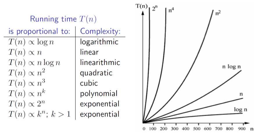
Recap: orders of growth
Factors which influence running time
- As well as the complexity of the particular sorting algorithm which is used, there are many other factors to consider which may have an effect on running time, e.g.
- How many items need to be sorted
- Are the items only related by the order relation, or do they have other restrictions (for example, are they all integers in the range 1 to 1000)
- To what extent are the items pre-sorted
- Can the items be placed into an internal (fast) computer memory or must they be sorted in external (slow) memory, such as on disk (so-called external sorting).
In-place sorting
- Sorting algorithms have different memory requirements, which depend on how the specific algorithm works.
- A sorting algorithm is called in-place if it uses only a fixed additional amount of working space, independent of the input size.
- Other sorting algorithms may require additional working memory, the amount of which is often related to the size of the input n
- In-place sorting is a desirable property if the availability of memory is a concern
Overview of sorting algorithms
| Algorithm | Best case | Worst case | Average case | Space Complexity | Stable? | |||
|---|---|---|---|---|---|---|---|---|
| Bubble Sort | <m>n</m> | <m>n | 2</m> | <m>n | 2</m> | 1 | Yes | |
| Selection Sort | <m>n | 2</m> | <m>n | 2</m> | <m>n | 2</m> | 1 | No |
| Insertion Sort | <m>n</m> | <m>n | 2</m> | <m>n | 2</m> | 1 | Yes | |
| Merge Sort | <m>n log n</m> | <m>n log n</m> | <m>n log n</m> | <m>O(n)</m> | Yes | |||
| Quicksort | <m>n log n</m> | <m>n | 2</m> | <m>n log n</m> | <m>n</m> (worst case) | No* | ||
| Heapsort | <m>n log n</m> | <m>n log n</m> | <m>n log n</m> | 1 | No | |||
| Counting Sort | <m>n + k</m> | <m>n + k</m> | <m>n + k</m> | <m>n + k</m> | Yes | |||
| Bucket Sort | <m>n + k</m> | <m>n | 2</m> | <m>n + k</m> | <m>n * k</m> | Yes | ||
| Timsort | <m>n</m> | <m>n log n</m> | <m>n log n</m> | <m>n</m> | Yes | |||
| Introsort | <m>n log n</m> | <m>n log n</m> | <m>n log n</m> | <m>log n</m> | No |
*the standard Quicksort algorithm is unstable, although stable variations do exist
Criteria for choosing a sorting algorithm
| Criteria | Sorting algorithm |
|---|---|
| Small number of items to be sorted | Insertion Sort |
| Items are mostly sorted already | Insertion Sort |
| Concerned about worst-case scenarios | Heap Sort |
| Interested in a good average-case behaviour | Quicksort |
| Items are drawn from a uniform dense universe | Bucket Sort |
| Desire to write as little code as possible | Insertion Sort |
| Stable sorting required | Merge Sort |
Week 9: Sorting Algorithms Part 2
Overview
- Review of sorting & desirable properties for sorting algorithms
- Introduction to simple sorting algorithms
- Bubble Sort
- Selection sort
- Insertion sort
Review of sorting
- Sorting - Arrange a collection of items according to pre-defined ordering rule
- Desirable properties for sorting algorithms
- Stability - preserve order of already sorted input
- Good run time efficiency(in the best, average or worst case)
- In-place sorting - if memory is a concern
- Suitability - the properties of the sorting algorithm are well-matched to the class of input instances which are expected i.e. consider specific strengths and weaknesses when choosing a sorting algorithm.
Overview of sorting algorithms
| Algorithm | Best case | Worst case | Average case | Space Complexity | Stable? | |||
|---|---|---|---|---|---|---|---|---|
| Bubble Sort | <m>n</m> | <m>n | 2</m> | <m>n | 2</m> | 1 | Yes | |
| Selection Sort | <m>n | 2</m> | <m>n | 2</m> | <m>n | 2</m> | 1 | No |
| Insertion Sort | <m>n</m> | <m>n | 2</m> | <m>n | 2</m> | 1 | Yes | |
| Merge Sort | <m>n log n</m> | <m>n log n</m> | <m>n log n</m> | <m>O(n)</m> | Yes | |||
| Quicksort | <m>n log n</m> | <m>n | 2</m> | <m>n log n</m> | <m>n</m> (worst case) | No* | ||
| Heapsort | <m>n log n</m> | <m>n log n</m> | <m>n log n</m> | 1 | No | |||
| Counting Sort | <m>n + k</m> | <m>n + k</m> | <m>n + k</m> | <m>n + k</m> | Yes | |||
| Bucket Sort | <m>n + k</m> | <m>n | 2</m> | <m>n + k</m> | <m>n * k</m> | Yes | ||
| Timsort | <m>n</m> | <m>n log n</m> | <m>n log n</m> | <m>n</m> | Yes | |||
| Introsort | <m>n log n</m> | <m>n log n</m> | <m>n log n</m> | <m>log n</m> | No |
*the standard Quicksort algorithm is unstable, although stable variations do exist
Comparison sorts
- A comparison sort is a type of sorting algorithm which uses comparison operations only to determine which of two elements should appear in a sorted list.
- A sorting algorithm is called comparison-based if the only way to gain information about the total order is by comparing a pair of elements at a time via the order ≤
- The simple sorting algorithms which we will discuss in this lecture (Bubble sort, insertion sort, and selection sort) all fall into this category.
- A fundamental result in algorithm analysis is that no algorithm that sorts by comparing elements can do better than <m>n</m> log <m>n</m> performance in the average or worst cases.
- Non-comparison sorting algorithms(e.g Bucket Sort, Counting Sort, Radix Sort) can have better worst-case times.
Bubble Sort
- Named for the way larger values in a list “Bubble up” to the end as sorting takes place
- Bubble sort was first analysed as early as 1956 (time complexity is <m>n</m> in best case, and <m>n^2</m> in worst and average cases)
- Comparison-based
- In-place sorting algorithm(i.e uses a constant amount of additional working space in addition to the memory required for the input)
- Simple to understand and implement, but it is slow and impractical for most problems even when compared to Insertion sort.
- Can be practical in some cases on data which is nearly sorted
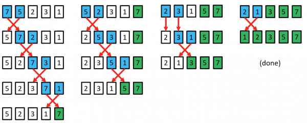
Bubble Sort procedure
- Compare each element(except the last one) with its neighbour to the right
- if they are out of order, swap them
- this puts the largest element at the very end
- the last element is now in the correct and final place
- Compare each element(except the last two) with its neighbour to the right
- If they are out of order, swap them
- This puts the second largest element next to last
- The last two elements are now in their correct and final places.
- Compare each element (except the last three) with its neighbour to the right
- …
- Continue as above until there are no unsorted elements on the left
Bubble Sort example
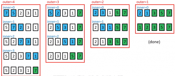
Bubble Sort in Code
public static void bubblesort(int[]a){
  int outer, inner;
  for(outer = a.length - 1; outer > 0;outer--){ //counting down
   for(inner=0;inner < outer;inner++){ //bubbling up
    if(a[inner] > a[inner+1];  { //if out of order....
    int temp = a[inner]; //...then swap
    a[inner] =a[inner+1];
    a[inner +1] = temp;
    }
   }
  }
 }
- bubblesort.py
# Bubble Sort in python
def printArray(arr):
  print (' '.join(str(i) for i in arr))


def bubblesort(arr):
  for i in range(len(arr)):
    for j in range(len(arr) - i - 1):
      if arr[j] > arr[j + 1]:
        temp = arr[j]
        arr[j] = arr[j + 1]
        arr[j + 1] = temp
    # Print array after every pass
    print ("After pass " + str(i) + "  :", printArray(arr))

if __name__ == '__main__':
    arr = [10, 7, 3, 1, 9, 7, 4, 3]
    print ("Initial Array :", printArray(arr))
    bubblesort(arr)
Bubble Sort Example
Analysing Bubble Sort (worst case)
for(outer =a.length-1; outer >0; outer--){
 for(inner=0; inner < outer; inner++){
  if(a[inner]>a[inner+1]){
  //swap code omitted
  }
 }
}
- In the worst case, the outer loop executes n-1 times (say n times)
- On average, inner loop executes about n/2 times for each outer loop
- In the inner loop, comparison and swap operations take constant time k
- Result is:
Selection Sort
- Comparison-based
- In-place
- Unstable
- Simple to implement
- Time complexity is <m>n^2</m> in best, worst and average cases.
- Generally gives better performance than Bubble Sort, but still impractical for real world tasks with a significant input size
- In every iteration of selection sort, the minimum element (when ascending order) from the unsorted subarray on the right is picked and moved to the sorted subarray on the left.
Selection Sort procedure
- Search elements 0 through n-1 and select the smallest
- swap it with the element in location 0
- Search elements 1 through n-1 and select the smallest
- swap it with the element in location 1
- Search elements 2 through n-1 and select the smallest
- swap it with the element in location 2
- Search elements 3 through n-1 and select the smallest
- swap it with the element in location 3
- Continue in this fashion until there's nothing left to search
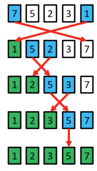
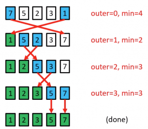
Selection Sort example
The element at index 4 is the smallest, so swap with index 0
The element at index 2 is the smallest, so swap with index 1
The element at index 3 is the smallest, so swap with index 2
The element at index 3 is the smallest, so swap with index 3
Selection sort might swap an array element with itself; this is harmless, and not worth checking for
Selection Sort in Code
public static void selectionsort(int[]a){
 int outer=0, inner=0, min=0;
 for(outer = 0; outer <a.length-1;outer++){  //outer counts up
 min = outer;
 for(inner = outer +1; inner <a.length; inner++){
  if(a[inner]<a[min]){ //find index of smallest value
   min = inner;
   }
  }
  //swap a [min] with a [outer]
  int temp = a[outer];
  a[outer] = a[min];
  a[min] = temp;
 }
}
- selection_sort.py
# selection sort in python
def printArray(arr):
  return (' '.join(str(i) for i in arr))


def selectionsort(arr):
  N = len(arr)
  for i in range(0, N):
    small = arr[i]
    pos = i
    for j in range(i + 1, N):
      if arr[j] < small:
        small = arr[j]
        pos = j
    temp = arr[pos]
    arr[pos] = arr[i]
    arr[i] = temp
    print ("After pass " + str(i) + "  :", printArray(arr))

if __name__ == '__main__':
    arr = [10, 7, 3, 1, 9, 7, 4, 3]
    print ("Initial Array :", printArray(arr))
    selectionsort(arr)
Analysing Selection Sort
- The outer loop runs <m>n</m> - 1 times
- The inner loop executes about <m>n</m>/2 times on average(from <m>n</m> to 2 times)
- Results is:
Insertion Sort
- Similar to the method usually used by card players to sort cards in their hand.
- Insertion sort is easy to implement, stable, in-place, and works well on small lists and lists that are close to sorted.
- On data sets which are already substantially sorted it runs in n +d time, where d is the number of inversions.
- However, it is very inefficient for large random lists.
- Insertion Sort is iterative and works by splitting a list of size n into a head(“sorted”) and tail(“unsorted”) sublist.
Insertion Sort procedure
- Start from the left of the array, and set the “key” as the element at index 1.Move any elements to the left which are > the “key” right by one position, and insert the “key”.
- Set the “Key” as the element at index 2. Move any elements to the left which are > the key right by one position and insert the key.
- Set the “key” as the element at the index 3. Move any elements to the left which are > the key right by one position and index the key.
- …
- Set the “key” as the elements at index <m>n</m>-1. Move any elements to the left which are > the key right by one position and insert the key.
- The array is now sorted.
Insertion Sort example
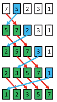
a[1]=5 is the key; 7>5 so move 7 right by one position, and insert 5 at index 0
a[2]=2 is the key; 7>2 so move both 7 and 5 right by one position, and insert 2 at index 0
a[3]=3 is the key; 7>3 and 5>3 so move both 7 and 5 right by one position, and insert 3 at index 1
a[4]=1 is the key; 7>1, 5>1, 3>1 and 2>1 so move both 7, 5, 3 and 2 right by one position, and insert 1 at index 1
(done)
Insertion Sort in code
public static void insertionsort(int a[]){
 for(int i=1; i<a.length; i++){
  int key =a[i]; //value to be inseted
  int j = i-1;
  //move all elements > key right one position
  while(j>=0 && a[j]>key){
  a[j+1]= a[j];
  j=j-1;
  }
  a[j+1]=key; //insert key in its new position
 }

}
- insertion_sort.py
# insertion sort
def printArray(arr):
  return(' '.join(str(i) for i in arr))


def insertionsort(arr):
  N = len(arr)
  for i in range(1, N):
    j = i - 1
    temp = arr[i]
    while j >= 0 and temp < arr[j]:
      arr[j + 1] = arr[j]
      j -= 1
    arr[j + 1] = temp
    print ("After pass " + str(i) + "  :", printArray(arr))

if __name__ == '__main__':
    arr = [10, 7, 3, 1, 9, 7, 4, 3]
    print ("Initial Array :", printArray(arr))
    insertionsort(arr)
Analysing Insertion Sort
- The total number of data comparisons made by insertion sort is the number of inversions d plus at most <m>n</m> -1
- A sorted list has no inversions - therefore insertion sort runs in linear Ω(n) time in the best case(when the input is already sorted)
Comparison of Simple sorting algorithms
- The main advantage that Insertion sort has over Selection Sort is that the inner loop only iterates as long as is necessary to find the insertion point.
- In the worst case, it will iterate over the entire sorted part. In the case, the number of iterations is the same as for selection sort and bubble sort.
- At the other extreme, however, if the array is already sorted, the inner loop won't need to iterate at all. In this case, the running time is Ω(n), which is the same as the running time of Bubble sort on an array which is already sorted.
- Bubble Sort, Selection sort and insertion sort are all in-place sorting algorithms.
- Bubble sort and insertion sort are stable, whereas selection sort
Criteria for choosing a sorting algorithm
| Criteria | Sorting algorithm |
|---|---|
| Small number of items to be sorted | Insertion Sort |
| Items are mostly sorted already | Insertion Sort |
| Concerned about worst-case scenarios | Heap Sort |
| Interested in a good average-case behaviour | Quicksort |
| Items are drawn from a uniform dense universe | Bucket Sort |
| Desire to write as little code as possible | Insertion Sort |
| Stable sorting required | Merge Sort |
Recap
- Bubble sort, selection sort and insertion sort are all O(<m>n^2</m>) in the worst case
- It is possible to do much better than this even with comparison-based sorts, as we will see in the next lecture
- from this lectuure on simple O(<m>n^2</m>)sorting algorithms:
- Bubble sort is extremely slow, and is of little practical use
- Selection sort is generally better than Bubble sort
- Selection sort and insertion sort are “good enough” for small input instances
- Insertion sort is usually the fastest of the three. In fact, for small <m>n</m> (say 5 or 10 elements), insertion sort is usually fasters than more complex algorithms.
Week 10: Sorting Algorithms Part 3
Overview
- Efficient comparison sort
- Merge sort
- Quick sort
- Non-comparison sorts
- Counting sort
- Bucket sort
- Hybrid Sorting algorithms
- Introsort
- Timsort
Overview of sorting algorithms
| Algorithm | Best case | Worst case | Average case | Space Complexity | Stable? | |||
|---|---|---|---|---|---|---|---|---|
| Bubble Sort | <m>n</m> | <m>n | 2</m> | <m>n | 2</m> | 1 | Yes | |
| Selection Sort | <m>n | 2</m> | <m>n | 2</m> | <m>n | 2</m> | 1 | No |
| Insertion Sort | <m>n</m> | <m>n | 2</m> | <m>n | 2</m> | 1 | Yes | |
| Merge Sort | <m>n log n</m> | <m>n log n</m> | <m>n log n</m> | <m>O(n)</m> | Yes | |||
| Quicksort | <m>n log n</m> | <m>n | 2</m> | <m>n log n</m> | <m>n</m> (worst case) | No* | ||
| Heapsort | <m>n log n</m> | <m>n log n</m> | <m>n log n</m> | 1 | No | |||
| Counting Sort | <m>n + k</m> | <m>n + k</m> | <m>n + k</m> | <m>n + k</m> | Yes | |||
| Bucket Sort | <m>n + k</m> | <m>n | 2</m> | <m>n + k</m> | <m>n * k</m> | Yes | ||
| Timsort | <m>n</m> | <m>n log n</m> | <m>n log n</m> | <m>n</m> | Yes | |||
| Introsort | <m>n log n</m> | <m>n log n</m> | <m>n log n</m> | <m>log n</m> | No |
*the standard Quicksort algorithm is unstable, although stable variations do exist
Merge sort
- Proposed by john von Neumann in 1945
- This algorithm exploits a recursive divide-and conquer approach resulting in a worst-case running time of 𝑂(<m>n log n</m> ), the best asymptotic behaviour which we have seen so far.
- It's best, worst, and average cases are very similar, making it a very good choice if predictable runtime is important - Merge Sort gives good all-round performance.
- Stable sort
- Versions of merge Sort are particularly good for sorting data with slow access times, such as data that cannot be held in internal memory(RAM) or are stored in linked lists.
Merge Sort Example
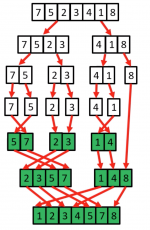
- Mergesort is based on the following basic idea:
- if the size of the list is 0 or 1, return.
- Otherwise, separate the list into two lists of equal or nearly equal size and recursively sort the first and second halves separately.
- finally, merge the two sorted halves into one sorted list.
- Clearly, almost all the work is in the merge step, which should be as efficient as possible.
- Any merge must take at least time that is linear in the total size of the two lists in the worst case, since every element must be looked at in order to determine the correct ordering.
Merge Sort in code
- merge_sort.py
- # Merge sort
- def mergesort(arr, i, j):
- mid = 0
- if i < j:
- mid = int((i + j) / 2)
- mergesort(arr, i, mid)
- mergesort(arr, mid + 1, j)
- merge(arr, i, mid, j)
- def merge(arr, i, mid, j):
- print ("Left: " + str(arr[i:mid + 1]))
- print ("Right: " + str(arr[mid + 1:j + 1]))
- N = len(arr)
- temp = [0] * N
- l = i
- r = j
- m = mid + 1
- k = l
- while l <= mid and m <= r:
- if arr[l] <= arr[m]:
- temp[k] = arr[l]
- l += 1
- else:
- temp[k] = arr[m]
- m += 1
- k += 1
- while l <= mid:
- temp[k] = arr[l]
- k += 1
- l += 1
- while m <= r:
- temp[k] = arr[m]
- k += 1
- m += 1
- for i1 in range(i, j + 1):
- arr[i1] = temp[i1]
- print ("After Merge: " + str(arr[i:j + 1]))
- if __name__ == '__main__':
- arr = [9, 4, 8, 3, 1, 2, 5]
- print ("Initial Array: " + str(arr))
- mergesort(arr, 0, len(arr) - 1)
Terminal Output:
Initial Array: [9, 4, 8, 3, 1, 2, 5]
Left: [9]
Right: [4]
After Merge: [4, 9]
Left: [8]
Right: [3]
After Merge: [3, 8]
Left: [4, 9]
Right: [3, 8]
After Merge: [3, 4, 8, 9]
Left: [1]
Right: [2]
After Merge: [1, 2]
Left: [1, 2]
Right: [5]
After Merge: [1, 2, 5]
Left: [3, 4, 8, 9]
Right: [1, 2, 5]
After Merge: [1, 2, 3, 4, 5, 8, 9]
Quicksort
- Developed by C.A.R Hoare in 1959
- Like Merge SORT, Quicksort is a recursive Divide and Conquer algorithm
- Standard version is not stable although stable versions do exist
- Performance: worst case <m>n^2</m> (rare), average case <m>n log n</m>, best case <m>n log n</m>
- Memory usage: O(<m>n</m>) (variants exist with O (n log n))
- In practice it is one of the fastest known sorting algorithms, on average
Quicksort procedure
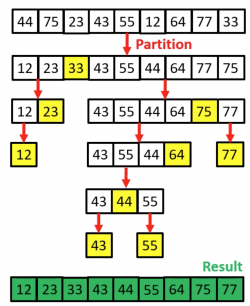
The main steps in Quick sort are:
- Pivot selection: Pick an element, called a “pivot” from the array
- Partioning: reorder the array elements with values < the pivot come beofre it, which all elements the values ≥ than the pivot come after it. After this partioining, the pivot is in its final position.
- Recursion: apply steps 1 and 2 above recursively to each of the two subarrays
The base case for the recursion is a subarray of length 1 or 0; by definition these cases do not need to be sorted.
Quicksort example
- On overage quicksort runs in <m>n</m> log <m>n</m> but if it consistently chooses bad pivots, its performance degrades to <m>n^2</m>.
- This happens if the pivot is consistently chosen so that all(or too many of) the elements in the array are < the pivot or > than the pivot. (A classic case is when the first or last element is chosen as a pivot and the data is already sorted, or nearly sorted).
- Some options for choosing the pivot:
- Always pick the first elements as the pivot.
- Always pick the last elements as the pivot.
- Pick a random element as the pivot.
- Pick the median element as the pivot.
Quick Sort Code
- quick_sort.py
- # Quick Sort
- def printArray(arr):
- return (' '.join(str(i) for i in arr))
- def quicksort(arr, i, j):
- if i < j:
- pos = partition(arr, i, j)
- quicksort(arr, i, pos - 1)
- quicksort(arr, pos + 1, j)
- def partition(arr, i, j):
- #pivot = arr[j] # pivot on the last item
- pivot = arr[int(j/2)] # pivot on the median
- small = i - 1
- for k in range(i, j):
- if arr[k] <= pivot:
- small += 1
- swap(arr, k, small)
- swap(arr, j, small + 1)
- print ("Pivot = " + str(arr[small + 1]), " Arr = " + printArray(arr))
- return small + 1
- def swap(arr, i, j):
- arr[i], arr[j] = arr[j], arr[i]
- if __name__ == '__main__':
- arr = [9, 4, 8, 3, 1, 2, 5]
- print (" Initial Array :",printArray(arr))
- quicksort(arr, 0, len(arr) - 1)
 Initial Array : 9 4 8 3 1 2 5
Pivot = 5  Arr = 4 3 1 2 5 9 8
Pivot = 2  Arr = 1 2 4 3 5 9 8
Pivot = 3  Arr = 1 2 3 4 5 9 8
Pivot = 8  Arr = 1 2 3 4 5 8 9
Non-comparison Sorts
- “Comparison sorts” make no assumptions about the data and compare all elements against each other (majority of sorting algortihms work in this way, including all sorting algorithms which we have discussed so far).
- 𝑂(<m>n</m> log <m>n</m>) time is the ideal “worst-case” scenario for a comparison-based sort (i.e 𝑂(<m>n</m> log <m>n</m>)) is the smallest penalty you can hope for in the worst case). Heapsort has this behaviour.
- <m>O(n)</m> time is possible if we make assumptions about the data and don't need to compare elements against each other (i.e., we know that data falls into a certain range or has some distribution).
- Example of non-comparison sorts including Counting sort, Bucket and Radix Sort.
- <m>O(n)</m> clearly is the minimum sorting time possible, since we must examine every element at least once (how can you sort an item you do not even examine?).
Counting Sort
- Proposed by Harold H.Seward in 1954.
- Counting Sort allows us to do something whihch seems impossible - sort a collection of items in (close to) linear time.
- How is this possible? Several assumptions must be made about the types of input instances which the algorithms will have to handle.
- i.e assume an input of size <m>n</m>, where each item has a non-negative integer key, with a range of k(if using zero-indexing, the keys are in the range [0,…,k-1])
- Best-, worst- and average-case time complexity of n +k, space complexity is also n+k
- The potential running time advantage comes at the cost of having an algorithm which is not a widely applicable as comparison sorts.
- Counting sort is stable(if implemented in the correct way!)
Counting Sort procedure
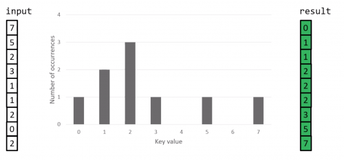
- Determine key range k in the input array(if not already known)
- Initialise an array count size k, which will be used to count the number of times that each key value appears in the input instance.
- Initialise an array result of size n, which will be used to store the sorted output.
- Iterate through the input array, and record the number of times each distinct key values occurs in the input instance.
- Construct the sorted result array, based on the histogram of key frequencies stored in count. Refer to the ordering of keys in input to ensure that stability is preserved.
Counting Sort example
Counting Sort Code
- counting_sort.py
- # Counting sort
- def printArray(arr):
- return(' '.join(str(i) for i in arr))
- def countingsort(arr):
- count = [0] * 11 # can store the count of positive numbers <= 10
- N = len(arr)
- for i in range(0, N):
- count[arr[i]] += 1
- for i in range(1, len(count)):
- count[i] += count[i - 1]
- print ("Counting Array :",
- printArray(count))
- output = [0] * N
- for i in range(len(arr)):
- output[count[arr[i]] - 1] = arr[i]
- count[arr[i]] -= 1
- print ("After Sorting :",
- printArray(output))
- if __name__ == '__main__':
- arr = [10, 7, 3, 1, 9, 7, 4, 3]
- print ("Initial Array :",
- printArray(arr))
- countingsort(arr)
Initial Array   : 10 7 3 1 9 7 4 3
Counting Array  : 0 1 1 3 4 4 4 6 6 7 8
After Sorting   : 1 3 3 4 7 7 9 10
Bucket Sort
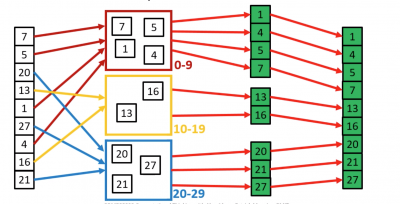
- Bucket sort is stable sort which works by distributing the elements of an array into a series of buckets. Each bucket is then sorted individually, either using a different sorting algorithm, or by recursively applying the bucket sort algorithm.
- Bucket sort can be seen as generalization of counting osrt; in fact, if each bucket has size 1 then bucket sort degenerates to counting sort.
- Time complexity is <m>n^2</m> in the worst case, and <m>n</m>+k in the best and average cases(where k is the number of buckets)
- Worst case space complexity is 𝑂(<m>n</m> + k)
- Bucket sort is useful when input values are uniformly distributed over a range e.g when sorting a large set of floating point numbers which values are uniformly distributed between 0.0 and 1.0
- Bucket Sort's performance degrades with clustering; if many values occur close together, they will all fall into a single buckets and be sorted slowly.
Bucket Sort procedure
- Set up an array of “Buckets”, which are initially empty
- Iterate through the input array, placing each element into its correct buckets
- Sort each non-empty bucket (using either a recursive call to bucket sort, or a different sorting algorithm e.g Insertion Sort)
- Visit the buckets in order, and place each elements back into its correct position.
Bucket Sort example
Hybrid Sorting Algorithms
- A hybrid algorithm is one which combines two or more algorithms which are designed to solve the same problem.
- Either chooses one specific algorithms depending on the data and execution conditions, or switches between different algorithms according to some rule set.
- Hybrid algorithms aim to combine the desired features of each constituent algorithms, to achieve a better algorithm in aggregate.
- E.g The best versions of Quicksort perform better than either Heap Sort or Merge Sort on the vast majority of inputs. However, Quicksort has poor worst-case running time (𝑂(<m>n^2</m>)) and <m>O(n)</m> stack usage. By comparison, both Heap sort and Merge Sort have 𝑂(<m>n log n</m>) worst-case running time, together with a stack usage of 𝑂(1) for Heap Sort or <m>O(n)</m> for Merge Sort. Furthermore, Insertion Sort performs better than any of these algorithms on small data sets.
Introsort
- Hybrid sorting algorithms proposed by David Musser in 1997.
- Variation of Quicksort which monitors the recursive depth of the standard Quicksort algorithm to ensure efficient processing.
- If the depth of the quicksort recursion exceeds <m>log n</m> levels, then Introsort switches to Heap sort instead.
- Since both algorithms which it uses are comparison-based, IntroSort is also comparison-based.
- Fast average- and worst-case performance i.e. <m>n log n</m>
Timsort
- Hybrid sorting algorithm Implemented by Tim Peters in 2002 for use in the python language.
- Derived from a combination of merge Sort and insertion sort, along with additional logic (including binary search)
- Finds subsequences (runs) of the data that are already ordered, and uses that knowledge to sort the reminder more efficiently, by merging an identified run with existing runs until certain criteria are fulfilled.
- Used on the android platform, python(since 2.3) for arrays of primitive type in Java SE 7, and in the GNU Octave software.
Criteria for choosing a sorting algorithm
| Criteria | Sorting algorithm |
|---|---|
| Small number of items to be sorted | Insertion Sort |
| Items are mostly sorted already | Insertion Sort |
| Concerned about worst-case scenarios | Heap Sort |
| Interested in a good average-case behaviour | Quicksort |
| Items are drawn from a uniform dense universe | Bucket Sort |
| Desire to write as little code as possible | Insertion Sort |
| Stable sorting required | Merge Sort |
Conclusion
- As we have seen, there are many different sorting algorithms, each of which has it own specific strengths and weaknesses.
- Comparison-based sorts are the most widely applicable; but are limited to <m>n log n</m> running time in the best case
- Non-Comparison sorts can achieve linear <m>n</m> running time in the best case, but are less flexible
- Hybrid sorting algorithms allow us to leverage the strengths of two or more algorithms (e.g. Timsort = Merge sort + insertion sort)
- There is no single algorithm which is best for all input instances; therefore it is important to use what you know about the expected input when choosing an algorithm.

