Table of Contents
Week 11 - Searching Algorithms
Overview
- The Search Problem
- Performance of Search Algorithms
- Types of Search Algorithms
- Linear Search (& how to beat it)
- Binary Search
The Search Problem
- Searching is a fundamental operation in computing.
- E.g. finding information on the web, looking up a bank account balance, finding a file or application on a PC, querying a database…
- The Search Problem relates to retrieving information from a data structure (e.g. Arrays, Linked Lists, Search Trees, Hash Tables etc.).
- Algorithms which solve the Search Problem are called Search Algorithms.
- Includes algorithms which query a data structure, such as the SQL SELECT command.
- Two fundamental queries about any collection C:
- Existence: Does C contain a target element? Given a collection C, we often simply want to know whether the collection already contains a given element t. The response to such a query is true if an element exists in the collection that matches the desired target t, or false if this is not the case.
- Associative lookup: Return information associated in collection C with a target key value k. A key is usually associated with a complex structure called a value. The lookup retrieves or replaces this value.
- A correct Search Algorithm should return true or the index of the requested key if it exists in the collection, or -1/null/false if it does not exist in the collection.
Reference: Pollice G., Selkow S. and Heineman G. (2016). Algorithms in a Nutshell, 2nd Edition. O' Reilly.
Performance of Search Algorithms
- Ultimately the performance of a Search Algorithm is based on how many operations performed (elements the algorithm inspects) as it processes a query (as we saw with Sorting Algorithms).
- Constant <m>O(n)</m> time is the worst case for any (reasonable) searching algorithm – corresponds to inspecting each element in a collection exactly once.
- As we will see, sorting a collection of items according to a comparator function (some definition of “less than”) can improve the performance of search queries.
- However, there are costs associated with maintaining a sorted collection, especially for use cases where frequent insertion or removal of keys/elements is expected.
- Trade-off between cost of maintaining a sorted collection, and the increased performance which is possible because of maintaining sorted data.
- Worth pre-sorting the collection if it will be searched often.
Pre-sorted data
- Several search operations become trivial when we can assume that a collection of items is sorted.
- E.g. Consider a set of economic data, such as the salary paid to all employees of a company. Values such as the minimum, maximum, median and quartile salaries may be retrieved from the data set in constant <m>O(1)</m> time if the data is sorted.
- Can also apply more advanced Search Algorithms when data is presorted.
Types of Search Algorithms
- Linear: simple (naïve) search algorithm
- Binary: better performance than Linear
- Comparison: eliminate records based on comparisons of record keys
- Digital: based on the properties of digits in record keys
- Hash-based: maps keys to records based on a hashing function
As we saw with Sorting Algorithms, there is no universal best algorithm for every possible use case. The most appropriate search algorithm often depends on the data structure being searched, but also on any a priori knowledge about the data.
Note: Only linear and binary covered in this module.
Linear Search
- Linear Search (also known as Sequential Search) is the simplest Searching Algorithm; it is trivial to implement.
- Brute-force approach to locate a single target value in a collection.
- Begins at the first index, and inspects each element in turn until it finds the target value, or it has inspected all elements in the collection.
- It is an appropriate algorithm to use when we do not know whether input data is sorted beforehand, or when the collection to be searched is small.
- Linear Search does not make any assumptions about the contents of a collection; it places the fewest restrictions on the type of elements which may be searched.
- The only requirement is the presence of a match function (some definition of “equals”) to determine whether the target element being searched for matches an element in the collection.
- Perhaps you frequently need to locate an element in a collection that may or may not be ordered.
- With no further knowledge about the information that might be in the collection, Linear Search gets the job done in a brute-force manner.
- It is the only search algorithm which may be used if the collection is accessible only through an iterator.
- Constant O(1) time in the best case, linear O(𝑛) time in the average and worst cases. Assuming that it is equally likely that the target value can be found at each array position, if the size of the input collection is doubled, the running time should also approximately double.
- Best case occurs when the element sought is at the first index, worst case occur when the element sought is at the last index, average case occurs when the element sought is somewhere in the middle.
- Constant space complexity.
Linear Search examples
Search the array a for the target value 7:
- a[0] = 2; this is not the target value, so continue
- a[1] = 1; this is not the target value, so continue
- a[2] = 5; this is not the target value, so continue
- a[3] = 4; this is not the target value, so continue
- a[4] = 8; this is not the target value, so continue
- a[5] = 7; this is the target value, so return index 5
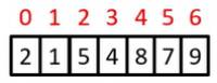
Search the array a for the target value 3:
- a[0] = 2; this is not the target value, so continue
- a[1] = 1; this is not the target value, so continue
- a[2] = 5; this is not the target value, so continue
- a[3] = 4; this is not the target value, so continue
- a[4] = 8; this is not the target value, so continue
- a[5] = 7; this is not the target value, so continue
- a[6] = 9; this is not the target value, so continue
- Iteration is complete. Target value was not found so return -1
Linear Search in code
- linear_search.py
- # Searching an element in a list/array in python
- # can be simply done using \'in\' operator
- # Example:
- # if x in arr:
- # print arr.index(x)
- # If you want to implement Linear Search in python
- # Linearly search x in arr[]
- # If x is present then return its location
- # else return -1
- def search(arr, x):
- for i in range(len(arr)):
- if arr[i] == x:
- return i
- return -1
Binary Search
- Linear Search has linear time complexity:
- Time <m>n</m> if the item is not found
- Time <m>n/2</m>, on average, if the item is found
- If the array is sorted, faster searching is possible
- How do we look up a name in a phone book, or a word in a dictionary?
- Look somewhere in the middle
- Compare what’s there with the target value that you are looking for
- Decide which half of the remaining entries to look at
- Repeat until you find the correct place
- This is the Binary Search Algorithm
- Better than linear running time is achievable only if the data is sorted in some way (i.e. given two index positions, i and j, a[i] < a[j] if and only if i < j).
- Binary Search delivers better performance than Linear Search because it starts with a collection whose elements are already sorted.
- Binary Search divides the sorted collection in half until the target value is found, or until it determines that the target value does not exist in the collection.
- Binary Search divides the collection approximately in half using whole integer division (i.e. 7/4 = 1, where the remainder is disregarded).
- Binary Search has logarithmic time complexity and constant space complexity.
Binary Search examples
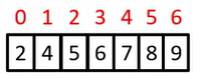
Search the array a for the target value 7:
- Middle index =(0+6)/2 = 3. a[3] = 6 < 7, so search in the right subarray (indices left=4 to right=6)
- Middle index =(4+6)/2 = 5. a[5] = 8 > 7, so search in the left subarray (indices left=4 to right=4)
- Middle index =(4+4)/2 = 4. a[4] = 7 = 7, so return index 4
Search the array a for the target value 3:
- Middle index =(0+6)/2 = 3. a[3] = 6 > 3, so search next in the left subarray (indices left=0 to right=2)
- Middle index =(0+2)/2 = 1. a[1] = 4 > 3, so search next in the left subarray (indices left=0 to right=1)
- Middle index =(0+1)/2 = 0. a[0] = 2 < 3, so search next in the right subarray (indices left=0 to right=0)
- Middle index =(0+0)/2 = 0. a[0] = 2 < 3. Now there is just one element left in the partition (index 0) – this corresponds to one of two possible base cases. Return -1 as this element is not the target value.
Iterative Binary Search in Code
- iterative_binary_search.py
- # Iterative Binary Search Function
- # It returns location of x in given array arr if present,
- # else returns -1
- def binarySearch(arr, l, r, x):
- while l <= r:
- mid = l + (r - l)/2;
- # Check if x is present at mid
- if arr[mid] == x:
- return mid
- # If x is greater, ignore left half
- elif arr[mid] < x:
- l = mid + 1
- # If x is smaller, ignore right half
- else:
- r = mid - 1
- # If we reach here, then the element was not present
- return -1
- # Test array
- arr = [ 2, 3, 4, 10, 40 ]
- x = 10
- # Function call
- result = binarySearch(arr, 0, len(arr)-1, x)
- if result != -1:
- print "Element is present at index %d" % result
- else:
- print "Element is not present in array"
Recursive Binary Search in Code
- recursive_binary_search.py
- # Python Program for recursive binary search.
- # Returns index of x in arr if present, else -1
- def binarySearch (arr, l, r, x):
- # Check base case
- if r >= l:
- mid = l + (r - l)/2
- # If element is present at the middle itself
- if arr[mid] == x:
- return mid
- # If element is smaller than mid, then it can only
- # be present in left subarray
- elif arr[mid] > x:
- return binarySearch(arr, l, mid-1, x)
- # Else the element can only be present in right subarray
- else:
- return binarySearch(arr, mid+1, r, x)
- else:
- # Element is not present in the array
- return -1
- # Test array
- arr = [ 2, 3, 4, 10, 40 ]
- x = 10
- # Function call
- result = binarySearch(arr, 0, len(arr)-1, x)
- if result != -1:
- print "Element is present at index %d" % result
- else:
- print "Element is not present in array"
Analysis of Binary Search
- In Binary Search, we choose an index that cuts the remaining portion of the array in half
- We repeat this until we either find the value we are looking for, or we reach a subarray of size 1
- If we start with an array of <m>size n</m>, we can cut it in half <m>log_2 n</m> times
- Hence, Binary Search has logarithmic <m>(log n)</m> time complexity in the worst and average cases, and constant time complexity in the best case
- For an array of size 1000, this is approx. 100 times faster than linear search (<m>2^10</m> ≈ 1000 when neglecting constant factors)
Conclusion
- Linear Search has linear time complexity
- Binary Search has logarithmic time complexity
- For large arrays, Binary Search is far more efficient than Linear Search
- However, Binary Search requires that the array is sorted
- If the array is sorted, Binary Search is
- Approx. 100 times faster for an array of size 1000 (neglecting constants)
- Approx. 50 000 times faster for an array of size 1 000 000 (neglecting constants)
- Significant improvements like these are what make studying and analysing algorithms worthwhile
Week 12: Benchmarking
Benchmarking Algorithms in Python
Overview
- Motivation for benchmarking
- Time in Python
- Benchmarking a single run
- Benchmarking multiple statistical runs
Motivation for Benchmarking
- Benchmarking or a posteriori analysis is an empirical method to compare the relative performance of algorithms implementations.
- Experimental (e.g running time) data may be used to validate theoretical or a priori analysis of algorithms
- Various hardware and software factors such system architecture, CPU design, choice of Operating System, background processes, energy saving and performance enhancing technologies etc. can effect running time.
- Therefore it is prudent to conduct multiple statistical runs using the same experimental setup, to ensure that your set of benchmarks are representative of the performance expected by an “average” user.
Time in Python
- Dates and times in Python are presented as the number of seconds that have elapsed since midnight on January 1st 1970 (the “unix epoch”)
- Each second since the Unix Epoch has a specific timestamp
- Can import the time module in Python to work with dates and times
- e.g start_time = time.time() # gets the current time in seconds
- e.g 15555001605 is Thursday, 11 April 2019 16:53:25 in GMT
Benchmarking a single run
import time

#log the start time in seconds
start_time = time.time()

#call the function you want to be benchmarked

#log the start time in seconds
end_time = time.time()

#calculate the elapsed time
time_elapsed = end_time - start_time
Benchmarking multiple statistical runs
import time

num_runs = 10 # number of times to test the function
results = [] # array to store the results for each test

# benchmark the function
for r in range(num_runs):
   # log the start time in seconds
   start_time = time.time()
   # call the function that you want to benchmark

   # log the end time in seconds
   end_time = time.time()

   # calculate the elapsed time
   time_elapsed = end_time - start_time

   results.append(time_elasped)
- benchmark.py
- from numpy.random import randint
- from time import time
- def Bubble_Sort(array):
- # your sort code
- sorted=array
- return sorted
- def Merge_Sort(array):
- # your sort code
- sorted=array
- return sorted
- def Counting_Sort(array):
- # your sort code
- sorted=array
- return sorted
- def Quick_Sort(array):
- # your sort code
- sorted=array
- return sorted
- def Timsort(array):
- # your sort code
- sorted=array
- return sorted
- # The actual names of your sort functions in your code somewhere, notice no quotes
- sort_functions_list = [Bubble_Sort, Merge_Sort, Counting_Sort, Quick_Sort, Timsort]
- # The prescribed array sizes to use in the benchmarking testst
- for ArraySize in (100, 250, 500, 750, 1000, 1250, 2500, 3750, 5000, 6250, 7500, 8750, 10000):
- # create a randowm array of values to use in the tests below
- testArray = randint(1,ArraySize*2,ArraySize)
- # iterate throug the list of sort functions to call in the test
- for sort_type in sort_functions_list:
- # and test every function ten times
- for i in range(10):
- start=time()
- sort_type(testArray)
- stop=time()
- print('{} {} {} {}'.format(sort_type, ArraySize, i, (stop-start)*1000))
Useful References
Python 3 time documentation: https://docs.python.org/3/library/time.html
Python Date and Time Overview https://www.tutorialspoint.com/python/python_date_time.htm
Discussions of benchmarking issues in Python (advanced material) https://www.peterbe.com/plog/how-to-do-performance-micro-benchmarks-in-python