help:statistics:distributions
Table of Contents
| DATA ANALYTICS REFERENCE DOCUMENT |
|
|---|---|
| Document Title: | A summary of statistical distributions |
| Document No.: | 1540297969 |
| Author(s): | Gerhard van der Linde |
| Contributor(s): | |
REVISION HISTORY
| Revision | Details of Modification(s) | Reason for modification | Date | By |
|---|---|---|---|---|
| 0 | Draft release | A Summary of distributions and what they do and look like | 2018/10/23 12:32 | Gerhard van der Linde |
Distributions

Distributions referenced below refers to the types of distrubutions discussed in probability2) theory and statistics3).
The purpose of this document attempt to provide a high level overview of each for reference and programming purposes. The list below is extracted from the numpy.random distributions documentation section.
Beta Distribution
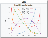 The beta distribution is a family of continuous probability distributions defined on the interval [0, 1] parametrized by two positive shape parameters, denoted by α and β, that appear as exponents of the random variable and control the shape of the distribution.
Binomial Distribution
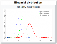 The binomial distribution with parameters n and p is the discrete probability distribution of the number of successes in a sequence of n independent experiments, each asking a yes–no question, and each with its own boolean-valued outcome: a random variable containing a single bit of information: success/yes/true/one (with probability p) or failure/no/false/zero (with probability q = 1 − p). A single success/failure experiment is also called a Bernoulli trial or Bernoulli experiment and a sequence of outcomes is called a Bernoulli process; for a single trial, i.e., n = 1, the binomial distribution is a Bernoulli distribution. The binomial distribution is the basis for the popular binomial test of statistical significance.
Chi-squared Distribution
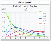 The chi-squared distribution (also chi-square or χ2-distribution) with k degrees of freedom is the distribution of a sum of the squares of k independent standard normal random variables. The chi-square distribution is a special case of the gamma distribution and is one of the most widely used probability distributions in inferential statistics, notably in hypothesis testing or in construction of confidence intervals. When it is being distinguished from the more general noncentral chi-squared distribution, this distribution is sometimes called the central chi-squared distribution.
Dirichlet Distribution
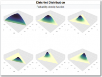 The Dirichlet distribution (after Peter Gustav Lejeune Dirichlet), often denoted Dir(α), is a family of continuous multivariate probability distributions parameterized by a vector α of positive reals. It is a multivariate generalization of the beta distribution. Dirichlet distributions are commonly used as prior distributions in Bayesian statistics, and in fact the Dirichlet distribution is the conjugate prior of the categorical distribution and multinomial distribution.
Exponential Distribution
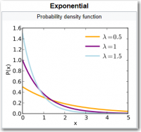 The exponential distribution (also known as the negative exponential distribution) is the probability distribution that describes the time between events in a Poisson point process, i.e., a process in which events occur continuously and independently at a constant average rate. It is a particular case of the gamma distribution. It is the continuous analogue of the geometric distribution, and it has the key property of being memoryless. In addition to being used for the analysis of Poisson point processes it is found in various other contexts.
Gamma Distribution
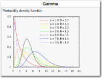 The gamma distribution is a two-parameter family of continuous probability distributions. The exponential distribution, Erlang distribution, and chi-squared distribution are special cases of the gamma distribution. There are three different parametrizations in common use:
1. With a shape parameter k and a scale parameter θ.
2. With a shape parameter α = k and an inverse scale parameter β = 1/θ, called a rate parameter.
3. With a shape parameter k and a mean parameter μ = kθ = α/β.
In each of these three forms, both parameters are positive real numbers.
Geometric Distribution
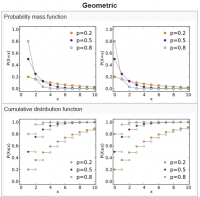 The geometric distribution is either of two discrete probability distributions:
The probability distribution of the number X of Bernoulli trials needed to get one success, supported on the set { 1, 2, 3, …}
The probability distribution of the number Y = X − 1 of failures before the first success, supported on the set { 0, 1, 2, 3, … }
Which of these one calls “the” geometric distribution is a matter of convention and convenience.
These two different geometric distributions should not be confused with each other. Often, the name shifted geometric distribution is adopted for the former one (distribution of the number X); however, to avoid ambiguity, it is considered wise to indicate which is intended, by mentioning the support explicitly.
The geometric distribution is either of two discrete probability distributions:
The probability distribution of the number X of Bernoulli trials needed to get one success, supported on the set { 1, 2, 3, …}
The probability distribution of the number Y = X − 1 of failures before the first success, supported on the set { 0, 1, 2, 3, … }
Which of these one calls “the” geometric distribution is a matter of convention and convenience.
These two different geometric distributions should not be confused with each other. Often, the name shifted geometric distribution is adopted for the former one (distribution of the number X); however, to avoid ambiguity, it is considered wise to indicate which is intended, by mentioning the support explicitly.
Gumbel Distribution
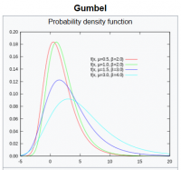 The Gumbel distribution (Generalized Extreme Value distribution Type-I) is used to model the distribution of the maximum (or the minimum) of a number of samples of various distributions. This distribution might be used to represent the distribution of the maximum level of a river in a particular year if there was a list of maximum values for the past ten years. It is useful in predicting the chance that an extreme earthquake, flood or other natural disaster will occur. The potential applicability of the Gumbel distribution to represent the distribution of maxima relates to extreme value theory, which indicates that it is likely to be useful if the distribution of the underlying sample data is of the normal or exponential type.
Reduced
Bernoulli and Uniform
You met the Bernoulli distribution above, over two discrete outcomes—tails or heads. Think of it, however, as a distribution over 0 and 1, over 0 heads (i.e. tails) or 1 heads. Above, both outcomes were equally likely, and that’s what’s illustrated in the diagram. The Bernoulli PDF38) has two lines of equal height, representing the two equally-probable outcomes of 0 and 1 at either end. The Bernoulli distribution could represent outcomes that aren’t equally likely, like the result of an unfair coin toss. Then, the probability of heads is not 0.5, but some other value p, and the probability of tails is 1-p. Like many distributions, it’s actually a family of distributions defined by parameters, like p here. When you think “Bernoulli,” just think “(possibly unfair) coin toss.” It’s a short jump to imagine a distribution over many equally-likely outcomes: the uniform distribution, characterized by its flat PDF. Imagine rolling a fair die. The outcomes 1 to 6 are equally likely. It can be defined for any number of outcomes n or even as a continuous distribution. Associate the uniform distribution with “rolling a fair die.”
Binomial and Hypergeometric
The binomial distribution may be thought of as the sum of outcomes of things that follow a Bernoulli distribution. Toss a fair coin 20 times; how many times does it come up heads? This count is an outcome that follows the binomial distribution. Its parameters are n, the number of trials, and p, the probability of a “success” (here: heads, or 1). Each flip is a Bernoulli-distributed outcome, or trial. Reach for the binomial distribution when counting the number of successes in things that act like a coin flip, where each flip is independent and has the same probability of success. Or, imagine an urn with equal numbers of white and black balls. Close your eyes and draw a ball and note whether it is black, then put it back. Repeat. How many times did you draw a black ball? This count also follows a binomial distribution. Imagining this odd situation has a point, because makes it simple to explain the hypergeometric distribution. This is the distribution of that same count if the balls were drawn without replacement instead. Undeniably it’s a cousin to the binomial distribution, but not the same, because the probability of success changes as balls are removed. If the number of balls is large relative to the number of draws, the distributions are similar because the chance of success changes less with each draw. When people talk about picking balls from urns without replacement, it’s almost always safe to interject, “the hypergeometric distribution, yes,” because I have never met anyone who actually filled urns with balls and then picked them out, and replaced them or otherwise, in real life. (I don’t even know anyone who owns an urn.) More broadly, it should come to mind when picking out a significant subset of a population as a sample.
Poisson
What about the count of customers calling a support hotline each minute? That’s an outcome whose distribution sounds binomial, if you think of each second as a Bernoulli trial in which a customer doesn’t call (0) or does (1). However, as the power company knows, when the power goes out, 2 or even hundreds of people can call in the same second. Viewing it as 60,000 millisecond-sized trials still doesn’t get around the problem—many more trials, much smaller probability of 1 call, let alone 2 or more, but, still not technically a Bernoulli trial. However, taking this to its infinite, logical conclusion works. Let n go to infinity and let p go to 0 to match so that np stays the same. This is like heading towards infinitely many infinitesimally small time slices in which the probability of a call is infinitesimal. The limiting result is the Poisson distribution. Like the binomial distribution, the Poisson distribution is the distribution of a count—the count of times something happened. It’s parameterized not by a probability p and number of trials n but by an average rate λ, which in this analogy is simply the constant value of np. The Poisson distribution is what you must think of when trying to count events over a time given the continuous rate of events occurring. When things like packets arrive at routers, or customers arrive at a store, or things wait in some kind of queue, think “Poisson.”
Geometric and Negative Binomial
From simple Bernoulli trials arises another distribution. How many times does a flipped coin come up tails before it first comes up heads? This count of tails follows a geometric distribution. Like the Bernoulli distribution, it’s parameterized by p, the probability of that final success. It’s not parameterized by n, a number of trials or flips, because the number of failure trials is the outcome itself. If the binomial distribution is “How many successes?” then the geometric distribution is “How many failures until a success?” The negative binomial distribution is a simple generalization. It’s the number of failures until r successes have occurred, not just 1. It’s therefore parameterized also by r. Sometimes it’s described as the number of successes until r failures. As my life coach says, success and failure are what you define them to be, so these are equivalent, as long as you keep straight whether p is the probability of success or failure. If you need an ice-breaker, you might point out that the binomial and hypergeometric distributions are an obvious pair, but the geometric and negative binomial distributions are also pretty similar, and then say, “I mean, who names these things, am I right?”
Exponential and Weibull
Back to customer support calls: how long until the next customer calls? The distribution of this waiting time sounds like it could be geometric, because every second that nobody calls is like a failure, until a second in which finally a customer calls. The number of failures is like the number of the seconds that nobody called, and that’s almost the waiting time until the next call, but almost isn’t close enough. The catch this time is that the sum will always be in whole seconds, but this fails to account for the wait within that second until the customer finally called. As before, take the geometric distribution to the limit, towards infinitesimal time slices, and it works. You get the exponential distribution, which accurately describes the distribution of time until a call. It’s a continuous distribution, the first encountered here, because the outcome time need not be whole seconds. Like the Poisson distribution, it is parameterized by a rate λ. Echoing the binomial-geometric relationship, Poisson’s “How many events per time?” relates to the exponential’s “How long until an event?” Given events whose count per time follows a Poisson distribution, then the time between events follows an exponential distribution with the same rate parameter λ. This correspondence between the two distributions is essential to name-check when discussing either of them. The exponential distribution should come to mind when thinking of “time until event”, maybe “time until failure.” In fact, this is so important that more general distributions exist to describe time-to-failure, like the Weibull distribution. Whereas the exponential distribution is appropriate when the rate—of wear, or failure for instance—is constant, the Weibull distribution can model increasing (or decreasing) rates of failure over time. The exponential is merely a special case. Think of “Weibull” when the chat turns to time-to-failure.
Normal, Log-Normal, Student’s t, and Chi-squared
The normal distribution, or Gaussian distribution, is maybe the most important of all. Its bell shape is instantly recognizable. Like e, it’s a curiously particular entity that turns up all over, from seemingly simple sources. Take a bunch of values following the same distribution—any distribution—and sum them. The distribution of their sum follows (approximately) the normal distribution. The more things that are summed, the more their sum’s distribution matches the normal distribution. (Caveats: must be a well-behaved distribution, must be independent, only tends to the normal distribution.) The fact that this is true regardless of the underlying distribution is amazing. This is called the central limit theorem, and you must know that this is what it’s called and what it means, or you will be immediately heckled. In this sense, it relates to all distributions. However it’s particularly related to distributions of sums of things. The sum of Bernoulli trials follows a binomial distribution, and as the number of trials increases, that binomial distribution becomes more like the normal distribution. Its cousin the hypergeometric distribution does too. The Poisson distribution—an extreme form of binomial—also approaches the normal distribution as the rate parameter increases. An outcome that follows a log-normal distribution takes on values whose logarithm is normally distributed. Or: the exponentiation of a normally-distributed value is log-normally distributed. If sums of things are normally distributed, then remember that products of things are log-normally distributed. Student’s t-distribution is the basis of the t-test that many non-statisticians learn in other sciences. It’s used in reasoning about the mean of a normal distribution, and also approaches the normal distribution as its parameter increases. The distinguishing feature of the t-distribution are its tails, which are fatter than the normal distribution’s. If the fat-tail anecdote isn’t a hot enough take to wow your neighbor, go to its mildly-interesting back-story concerning beer. Over 100 years ago, Guinness was using statistics to make better stout. There, William Sealy Gosset developed some whole new stats theory just to grow better barley. Gosset convinced the boss that the other brewers couldn’t figure out how to use the ideas, and so got permission to publish, but only under the pen name “Student”. Gosset’s best-known result is this t-distribution, which is sort of named after him. Finally, the chi-squared distribution is the distribution of the sum of squares of normally-distributed values. It’s the distribution underpinning the chi-squared test which is itself based on the sum of squares of differences, which are supposed to be normally distributed.
Gamma and Beta
At this point, if you’re talking about chi-squared anything, then the conversation has gotten serious. You are likely talking to actual statisticians, and you may want to excuse yourself at this point, because things like the gamma distribution may come up. It is a generalization of both the exponential and chi-squared distributions. More like the exponential distribution, it is used as a sophisticated model of waiting times. For example, the gamma distribution comes up when modeling the time until the next n events occur. It appears in machine learning as the “conjugate prior” to a couple distributions. Do not get into that conversation about conjugate priors, but if you do, be sure that you’re about to talk about the beta distribution, because it’s the conjugate prior to most every other distribution mentioned here. As far as data scientists are concerned, that’s what it was built for. Mention this casually, and move toward the door.
help/statistics/distributions.txt · Last modified: 2020/06/20 14:39 by 127.0.0.1